Rat Cerebellum volume¶

This Use Case places cerebellar neurons (different types: specific simplified geometric features with anisotropic properties and specific density) into a layered-volume of the cerebellum. This Use Case can be found in Online Use Cases/Circuit Building/Cells placement/Rat cerebellum volume.

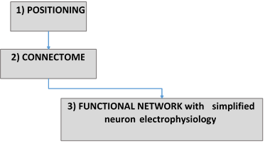
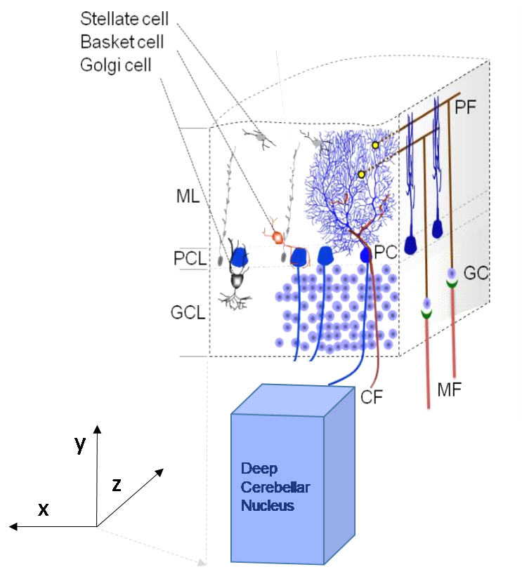
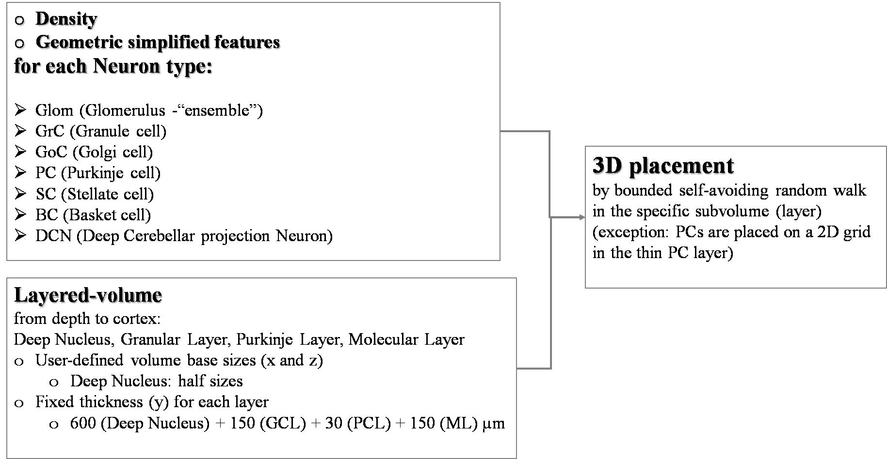
Approach: the desired number of cells are progressively placed following a random direction from the previous cell with a distance step guaranteeing that they do not overlap. A “reset” starting point occurs when the entire surrounding is occupied. This algorithm is computationally efficient, which is fundamental for high-density volumes, but still keeps a strong random component to achieve a realistic distribution of the pairwise inter-neuron distances. The PC Layer is almost a planar grid in-between GRL and ML, with an inter-soma distance along the x-axis constrained by the requirement that adjacent dendritic trees must not overlap.

Inputs: by a simple GUI, the basic parameters can be entered by the user

Base sizes (x and z) of the cerebellar volume to be built
Plot option enabling
Save option enabling

Expert users can modify more parameters from scaffold_params.py (in /storage):

Neuron types (with ID)
Simplified geometric features for each neuron type: radius of the soma, and eventually dendritic field extensions (direction-dependent) if the constraints of not-overlapping cells are taken into account
Density for each neuron type, and eventually the ratio of the density values when compagin different types.

Output:

hdf5 matrix with 5 columns (saved in /storage)
Neuron ID (unique)
Neuron type ID (from 1 to 7)
3D coordinates (soma center) of each neuron (x, y, and z)

Monitoring: sparseness in the subvolume by computing the distribution of pairwise distances (monitoring_positioning.py in /storage)

Moreover, a 3D basic visualization is depicted (somas of each neuron, using a different color for each neuron type).

Additional information:

The whole Use Case should take about 10 minutes for a volume base of 400 x 400 µm.
No log in to any other computer required.

EXAMPLE

x = 400 µm, z = 400 µm (→ DCN 200 x 200 µm)

y = 930 µm (600+ 150+30+150 µm), i.e. thickness DCN + GRL+ PCL + ML

TOT #NEURONS: 96.887

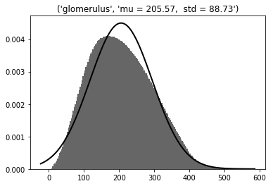
Glomeruli (N=7073, radius =1.5 µm, in GRL excluded the upper 10 µm)

3D dist = 206 ± 89 µm - Gaussian

Min = 4; max =558 µm

Granule cells (N=88229, radius = 2.5 µm, in the whole GRL)

3D dist = 210 ± 90 µm- Gaussian

Min = ; max = µm

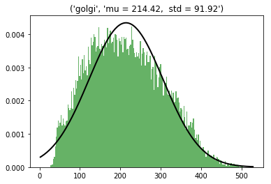
Golgi cells (N=219, radius = 8 µm, in GRL excluded the bottom 10 µm)

3D dist = 214 ± 91 µm – Gaussian

Min = 26; max =504 µm

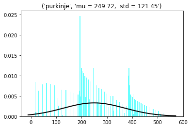
Purkinje cells (N=78, radius = 7.5 µm, in PCL, planar grid)

3D dist = 250 ± 121 µm

Min = 15; max =544 µm

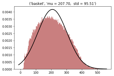
Basket cells (N=603, radius = 6 µm, in the ML lower half)

3D dist = 208 ± 96 µm - Gaussian

Min = 13; max = 534 µm

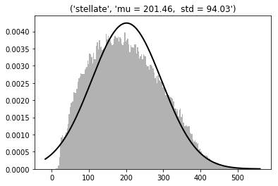
Stellate cells (N=603, radius = 4 µm, in the ML upper half)

3D dist = 201 ±94 µm - Gaussian

Min = 9; max = 534 µm

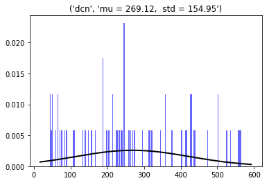
Deep Cerebellar projection Neurons (N=12, radius=10 µm, in the Deep Nucleus)

3D dist = 269 ± 155 µm

Min = 44; max = 566 µm